Physical Aspects of Nature

Resources for Physical Aspects of Nature - for more information about the course, please see course outlines.

Maths skills

There are several mathematical skills that will be useful for your Physics study. The following seminars and worksheets might help you to revise those skills.

Gaussian distributions and histograms

In one of the practicals in this course, you are required to draw a histogram with a Gaussian (normal) curve overlaid.
Here is some advice for doing that from MLC lecturer David.

About Gaussian distribution curves

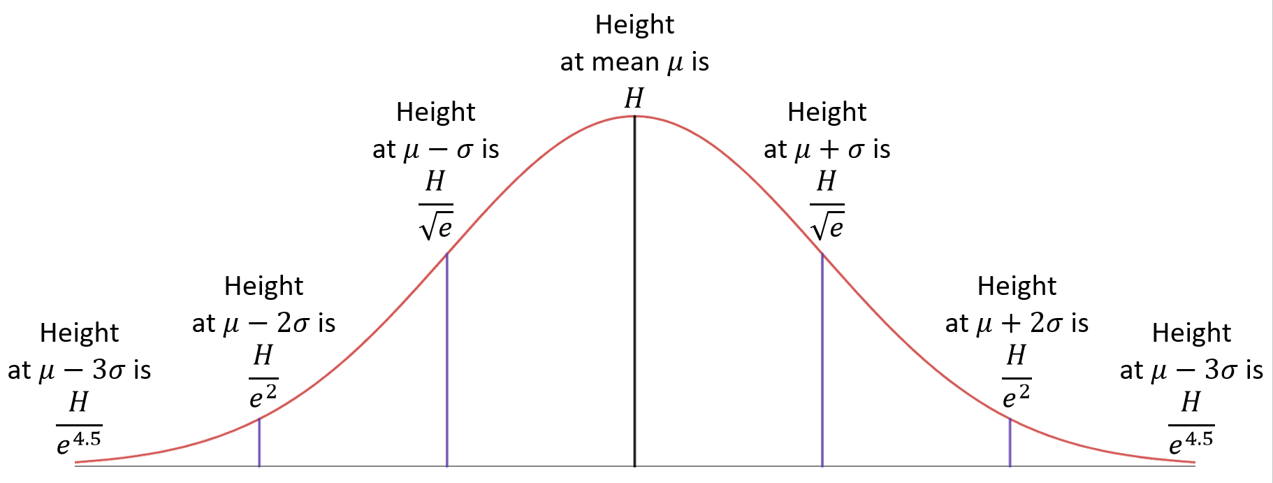
There is a formula for the height of the Gaussian distribution curve, but in order to draw a decent sketch of a Gaussian curve, you really only need the height at the mean (μ), at one standard deviation above and below the mean (μ+σ and μ-σ), at two standard deviations above and below the mean (μ+2σ and μ-2σ) and at three standard deviations above and below the mean (μ+3σ and μ-3σ) You can then draw a curve through those points.

The correct height at the mean is the area divided by σ√(2π), but it is okay for most purposes to choose any height that looks right to you.

This image shows a normal distribution with the formula for the height at the mean.

The correct height at both μ+σ and μ-σ is the height at the mean divided by √e. That is, approximately 61% of the height at the mean.
The correct height at both μ+2σ and μ-2σ is the height at the mean divided by e². That is, approximately 14% of the height at the mean.
The correct height at both μ+3σ and μ-3σ is the height at the mean divided by e⁴∙⁵. That is, approximately 1% of the height at the mean.

This image shows a normal distribution with formulas for the height at various distances from the mean.

This image shows a normal distribution with decimals to multiply the height at the mean to get the height at various distances from the mean.

Note that the number e is approximately 2.7182818284, and a scientific calculator will have this number programmed into it (just like it will have the number π programmed into it).

For your interest, the formula for a Gaussian curve with total area A goes like this: If (x-μ)/σ=k, then f(x)=A/[σ√(2π)]×e^[-1/2×k²].

About the computer simulation

The computer simulation for your prac will show you a list of bins and the frequency in each bin in order to draw a histogram.
You must write down the mean and standard deviation that the computer gives you before you get the histogram data.
It is impossible to figure out the exact correct mean and standard deviation from the histogram data alone!
You also need to change the number of bins and the maximum until you get the pictures on the screen to look they way you want, and then get it to show you the list of histogram data.

Drawing histograms with normal distributions using Excel

Making the histogram

Copy and paste the histogram data from the online prac simulation into excel.
Excel will draw its histogram with the numbers in the centre of each column, but the numbers in the data from the simulation are the left hand end of the column. So you will have to add half the bin width to each number in the Bins column.
For example, if your Bins column has 0, 20, 40, 60, ..., then you will need to change them to 10, 30, 50, 70, ...
Highlight just the column for number of observations, then click on "Insert > Chart > Column chart". Do not ask it to draw a histogram! It won't know how to deal with the kind of data you have if you ask it to draw a histogram. You have to select a Column Chart.
Once you have the graph, go to "Chart tools > Design > Select Data". In the box select "Horizontal (Category) Axis Labels > Edit" and then highlight the Bins column in the data.
Finally, click on the bars themselves and go to "Chart tools > Format > Format selection". Change the "Gap Width" to 0%. Also make the border a solid line with black colour and the fill a light colour.

Making the Gaussian curve

Excel is very bad at drawing smooth curves over the top of histograms! The easiest way to do it is to insert a transparent picture yourself over the top.

Download this png image file which is a picture of a Gaussian curve with a transparent background.
In Excel go to "Insert > Illustrations > Pictures" and find the file (called "normal-graph-transparent.png") and insert it.
Line up the black mean line with the mean on the x-axis.
Calculate the mean plus one standard deviation and find with your eyes where that place should be on the graph's x-axis.
For example, if the mean was 350 and the standard deviation was 23, you would calculate 350+23=373.
Hold down CRTL or COMMAND while dragging the handle on the right-hand side of the image until the purple mean-plus-standard-deviation line lines up with the correct spot on the x-axis.
Drag the handle on the top of the image until it looks like a good height.

Drawing histograms with normal distributions by hand

Making the histogram

Draw an x-axis with marks for the numbers in the "Bins" column of the data.
Between these marks, you will draw columns of heights to match the "N. Obs" column of the data. Each column will be to the right of the matching number in the Bins column.
For example, suppose the data table had 0, 20, 40 in the Bins column, and 1, 5, 10 in the N. Obs column
Then you would draw a column of height 1 between the 0 mark and the 20 mark, and you would draw a column of height 5 between the 20 mark and the 40 mark, and you would draw a column of height 10 between the 40 mark and the 60 mark.

Making the Gaussian curve

Calculate the mean plus and minus one standard deviation, and the mean plus and minus two standard deviations, and the mean plus and minus three standard deviations, and mark those places on the graph's x-axis.
For example, if the mean was 350 and the standard deviation was 23, you would calculate 350+23=373 and 350-23=327, and 350+2×23=396 and 350-2×23=304, and 350+3×23=419 and 350-3×23=281.
Calculate the area of the graph by multiplying the total number of observations times the bin width.
For example, if the Bins column was 0, 20, 40, 60, ... that would mean the bin width is 20 because those numbers are 20 apart.
If there were 43 observations total, the area would be 43×20=860.
Calculate the height for the curve at the mean by Area/[standard deviation × √(2π)]. Draw a line of that height at the mean.
For example, if the area was 860 and the standard deviation was 23, the height would be 860/(23×√(2π))= 14.9.
Calculate the height for the curve at one standard deviation from the mean by (Height at the mean)×0.61. Draw lines of that height at one standard deviation from the mean.
For example, if the height at the mean turned out to be 14.9, then the height at one standard deviation from the mean would be 14.9×0.61 = 9.0.
Calculate the height for the curve at two standard deviations from the mean by (Height at the mean)×0.14. Draw lines of that height at two standard deviations from the mean.
For example if the height at the mean turned out to be 14.9, then the height at one standard deviation from the mean would be 14.9×0.14 = 2.0.
Calculate the height for the curve three standard deviations from the mean by (Height at the mean)×0.01. Draw lines of that height at two standard deviations from the mean.
For example if the height at the mean turned out to be 14.9, then the height at one standard deviation from the mean would be 14.9×0.01 = 0.15, which is almost zero.
Connect the tops of those seven lines with a smooth Gaussian curve.

The MLC Drop-In Centre

If you have any questions about the above resources, or about any maths relating to your courses, please visit us in the MLC drop-in centre.